Sklearn Random Forest Classification
SKLearn Classification using a Random Forest Model
import platform
import sys

import pandas as pd
import numpy as np
from matplotlib import pyplot as plt
import matplotlib
matplotlib.style.use('ggplot')

%matplotlib inline

import time
from scipy.stats import randint as sp_randint
import seaborn as sns

import sklearn
from sklearn.preprocessing import OneHotEncoder
from sklearn.ensemble import RandomForestClassifier
from sklearn.mixture import GaussianMixture
from sklearn.model_selection import RandomizedSearchCV, GridSearchCV
from sklearn.model_selection import cross_val_score, train_test_split
from sklearn import metrics

from sklearn.metrics import roc_auc_score, roc_curve, auc, classification_report
from sklearn.metrics import f1_score, precision_score, recall_score
from sklearn.metrics import mean_squared_error, cohen_kappa_score, make_scorer
from sklearn.metrics import confusion_matrix, accuracy_score, average_precision_score
from sklearn.metrics import precision_recall_curve, SCORERS
from sklearn.model_selection import learning_curve
from sklearn.model_selection import ShuffleSplit
from sklearn.externals import joblib
from operator import itemgetter

from tabulate import tabulate
Here is the environment for this notebook
print('Operating system version....', platform.platform())
print("Python version is........... %s.%s.%s" % sys.version_info[:3])
print('scikit-learn version is.....', sklearn.__version__)
print('pandas version is...........', pd.__version__)
print('numpy version is............', np.__version__)
print('matplotlib version is.......', matplotlib.__version__)
Operating system version.... Windows-10-10.0.16299-SP0
Python version is........... 3.6.4
scikit-learn version is..... 0.19.1
pandas version is........... 0.22.0
numpy version is............ 1.13.3
matplotlib version is....... 2.1.2
Define a TIme Class to computer total execution time
class Timer:
  def __init__(self):
    self.start = time.time()

  def restart(self):
    self.start = time.time()

  def get_time(self):
    end = time.time()
    m, s = divmod(end - self.start, 60)
    h, m = divmod(m, 60)
    time_str = "%02d:%02d:%02d" % (h, m, s)
    return time_str
Define a correlation plot method
def Correlation_plot(df):
    plt.ioff()
    red_green = ["#ff0000", "#00ff00"]
    sns.set_palette(red_green)
    np.seterr(divide='ignore', invalid='ignore')
    g = sns.pairplot(df,
                     diag_kind = 'kde',
                     hue = 'Altitude',
                     markers = ["o", "D"],
                     size = 1.5,
                     aspect = 1,
                     plot_kws = {"s": 6})
    g.fig.subplots_adjust(right = 0.9)
    plt.show()
Define a method to load the Bottle Rocket Data Set
We load the Bottle Rocket data into two datasets: train and test. Since we are doing cross-validation, we only need the train dataset to do training. The test dataset is our “out-of-sample” data that will be used only after training is done. This is an attempt to simulate a production environment.
def LoadData():
    global X_train, y_train, X_test, y_test, train, test
    global feature_columns, response_column, n_features

    model_full = pd.read_csv("C:/sm/BottleRockets/model-8-1.csv")

    response_column = ['Altitude']
    feature_columns = ['BoxRatio','Thrust', 'Velocity', 'OnBalRun', 'vwapGain']
    n_features = len(feature_columns)
    mask = feature_columns + response_column

    model = model_full[mask]
    print('Model dataset:\n', model.head(5))
    print('\nDescription of model dataset:\n', model[feature_columns].describe(include='all'))

    Correlation_plot(model)

    # Split the data into Train and Test with Train having 80% and test 20% each
    train_full, test_full = np.split(model_full.sample(frac=1), [int(.8*len(model))])

    X_train  = train_full[feature_columns].as_matrix()
    y_train_ = train_full[response_column].as_matrix()
    X_test   = test_full[feature_columns].as_matrix()
    y_test_  = test_full[response_column].as_matrix()

    y_train = np.reshape(y_train_, len(y_train_))
    y_test  = np.reshape(y_test_,  len(y_test_))

    train = train_full[mask]
    test  = test_full[mask]
    print('Shape of train: ', train.shape)
    print('Shape of test:  ', test.shape)
    return
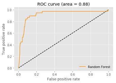
Define a method to plot a ROC Curve
def ROC_Curve(rf, auc):
    one_hot_encoder = OneHotEncoder()
    rf_fit = rf.fit(X_train, y_train)
    fit = one_hot_encoder.fit(rf.apply(X_train))
    y_predicted = rf.predict_proba(X_test)[:, 1]
    false_positive, true_positive, _ = roc_curve(y_test, y_predicted)

    plt.figure()
    plt.plot([0, 1], [0, 1], 'k--')
    plt.plot(false_positive, true_positive, color='darkorange', label='Random Forest')
    plt.xlabel('False positive rate')
    plt.ylabel('True positive rate')
    plt.title('ROC curve (area = %0.2f)' % auc)
    plt.legend(loc='best')
    plt.show()
Define a method to print the model performance
def Print_Metrics(saved_rf):
    print('\nModel performance on the test data set:')

    # print('Train Accuracy.......', accuracy_score(y_train, best_model.predict(X_train)))
    # print('Validate Accuracy....', accuracy_score(y_valid, best_model.predict(X_valid)))

    y_predict_test  = best_model.predict(X_test)
    mse             = metrics.mean_squared_error(y_test, y_predict_test)
    logloss_test    = metrics.log_loss(y_test, y_predict_test)
    accuracy_test   = metrics.accuracy_score(y_test, y_predict_test)
    accuracy_test2  = best_model.score(X_test, y_test)
    F1_test         = metrics.f1_score(y_test, y_predict_test)
    precision_test  = precision_score(y_test, y_predict_test, average='binary')
    precision_test2 = metrics.precision_score(y_test, y_predict_test)
    recall_test     = recall_score(y_test, y_predict_test, average='binary')
    auc_test        = metrics.roc_auc_score(y_test, y_predict_test)
    r2_test         = metrics.r2_score(y_test, y_predict_test)

    #test_auc       = h2o.get_model("best_rf").model_performance(test_data=test).auc()
    #print('Best model performance based on auc: ', test_auc)

    header = ["Metric", "Test"]
    table  = [
               ["logloss",   logloss_test],
               ["accuracy",  accuracy_test],
               ["precision", precision_test],
               ["F1",        F1_test],
               ["r2",        r2_test],
               ["AUC",       auc_test]
             ]

    print(tabulate(table, header, tablefmt="fancy_grid"))
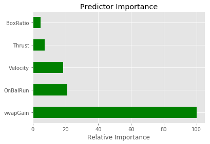
Define a method to plot the predictor importance
def Plot_predictor_importance(best_model, feature_columns):
    feature_importances = best_model.feature_importances_
    sorted_idx = np.argsort(feature_importances)
    y_pos  = np.arange(sorted_idx.shape[0]) + .5
    fig, ax = plt.subplots()
    ax.barh(y_pos,
            feature_importances[sorted_idx],
            align='center',
            color='green',
            ecolor='black',
            height=0.5)
    ax.set_yticks(y_pos)
    ax.set_yticklabels(feature_columns)
    ax.invert_yaxis()
    ax.set_xlabel('Relative Importance')
    ax.set_title('Predictor Importance')
    plt.show()
Define a utility function to report best scores
def Report_scores(results, n_top=3):
    for i in range(1, n_top + 1):
        candidates = np.flatnonzero(results['rank_test_score'] == i)
        for candidate in candidates:
            print("Model with rank: {0}".format(i))
            print("Mean validation score: {0:.3f} (std: {1:.3f})".format(
                  results['mean_test_score'][candidate],
                  results['std_test_score'][candidate]))
            print("Parameters: {0}".format(results['params'][candidate]))
            print("")
Define a method to print the Confusion Matrix and the performance metrics
def Print_confusion_matrix(cm, auc, heading):
    print('\n', heading)
    print(cm)
    true_negative  = cm[0,0]
    true_positive  = cm[1,1]
    false_negative = cm[1,0]
    false_positive = cm[0,1]
    total = true_negative + true_positive + false_negative + false_positive
    accuracy = (true_positive + true_negative)/total
    precision = (true_positive)/(true_positive + false_positive)
    recall = (true_positive)/(true_positive + false_negative)
    misclassification_rate = (false_positive + false_negative)/total
    F1 = (2*true_positive)/(2*true_positive + false_positive + false_negative)
    print('accuracy.................%7.4f' % accuracy)
    print('precision................%7.4f' % precision)
    print('recall...................%7.4f' % recall)
    print('F1.......................%7.4f' % F1)
    print('auc......................%7.4f' % auc)
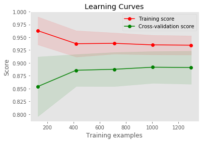
Plot the learning curves
def Plot_learning_curve(estimator, title, X, y, ylim = None, cv = None,
                        n_jobs = 1, train_sizes = np.linspace(0.1, 1.0, 5)):
    plt.figure()
    plt.title(title)
    if ylim is not None:
        plt.ylim(*ylim)
    plt.xlabel("Training examples")
    plt.ylabel("Score")
    train_sizes, train_scores, test_scores = learning_curve(estimator,
                                                            X, y,
                                                            cv = cv,
                                                            n_jobs = n_jobs,
                                                            train_sizes = train_sizes)
    train_scores_mean = np.mean(train_scores, axis=1)
    train_scores_std = np.std(train_scores, axis=1)
    test_scores_mean = np.mean(test_scores, axis=1)
    test_scores_std = np.std(test_scores, axis=1)
    plt.grid()

    plt.fill_between(train_sizes, train_scores_mean - train_scores_std,
                     train_scores_mean + train_scores_std, alpha=0.1,
                     color="r")
    plt.fill_between(train_sizes, test_scores_mean - test_scores_std,
                     test_scores_mean + test_scores_std, alpha=0.1, color="g")
    plt.plot(train_sizes, train_scores_mean, 'o-', color="r",
             label="Training score")
    plt.plot(train_sizes, test_scores_mean, 'o-', color="g",
             label="Cross-validation score")

    plt.legend(loc="best")
    plt.show()
    return
Define the hyperparameters for a random search
def Random_Search():
    global best_model, saved_moldel

    param_grid = {"n_estimators": range(20, 100, 2),
                  "max_depth": range(4, 50, 2),
                  "min_samples_leaf": range(2, 100, 2),
                  "max_features": sp_randint(1, n_features),
                  "min_samples_split": sp_randint(2, 10),
                  "bootstrap": [True, False],
                  "criterion": ["gini", "entropy"]}

    clf = RandomForestClassifier(class_weight = 'balanced')
    n_iter_search = 500
    estimator = RandomizedSearchCV(clf,
                                   param_distributions = param_grid,
                                   n_iter = n_iter_search,
                                   scoring = 'roc_auc',
                                   verbose = 0,
                                   n_jobs = 1)

    fit = estimator.fit(X_train, y_train)

    # Cross validation with 20 iterations to get smoother mean test and train
    # score curves, each time with 20% data randomly selected as a validation set.
    cv_ = ShuffleSplit(n_splits = 20, test_size = 0.20, random_state = 0)
    Plot_learning_curve(estimator,
                        'Learning Curves',
                        X_train, y_train,
                        cv = cv_,
                        n_jobs = 1)

    Report_scores(estimator.cv_results_, n_top = 3)

    best_model = estimator.best_estimator_
    print('\nbest_model:\n', best_model)

    print('\nFeature Importances:', best_model.feature_importances_)
    Plot_predictor_importance(best_model, feature_columns)

    y_predicted = best_model.predict(X_train)
    probabilities = best_model.predict_proba(X_train)

    c_report = classification_report(y_train, y_predicted)
    print('\nClassification report:\n', c_report)

    y_predicted_train = best_model.predict(X_train)
    cm = confusion_matrix(y_train, y_predicted_train)
    auc = roc_auc_score(y_train, y_predicted_train)
    Print_confusion_matrix(cm, auc, 'Confusion matrics of the training dataset')

    y_predicted = best_model.predict(X_test)
    cm = confusion_matrix(y_test, y_predicted)
    auc = roc_auc_score(y_test, y_predicted)

    ntotal = len(y_test)
    correct = y_test == y_predicted
    numCorrect = sum(correct)
    percent = round( (100.0*numCorrect)/ntotal, 6)
    print("\nCorrect classifications on test data: {0:d}/{1:d} {2:8.3f}%".format(numCorrect, ntotal, percent))
    prediction_score = 100.0*best_model.score(X_test, y_test)
    print('Random Forest Prediction Score on test data: %8.3f' % prediction_score)

    model_path = 'C:/sm/BottleRockets/trained_models/sklearn_rf_classify.pkl'
    joblib.dump(best_model, model_path)

    saved_model = joblib.load(model_path)
    y_predicted_test = best_model.predict(X_test)
    cm = confusion_matrix(y_test, y_predicted_test)
    auc = roc_auc_score(y_test, y_predicted_test)
    Print_confusion_matrix(cm, auc, 'Confusion matrics of the test dataset')
    ROC_Curve(best_model, auc)
    Print_Metrics(saved_model)
    return
Run the random search
my_timer = Timer()
LoadData()
Random_Search()
elapsed = my_timer.get_time()
print("\nTotal compute time was: %s" % elapsed)
Model dataset:
    BoxRatio  Thrust  Velocity  OnBalRun  vwapGain  Altitude
0     0.166   0.166     0.317     0.455    -0.068         0
1     0.071   0.068     0.170     0.482    -0.231         0
2    -0.031  -0.031     0.109     0.531     0.115         0
3    -0.186  -0.193     0.344     0.548     0.111         0
4    -0.147  -0.147     0.326     0.597     0.157         1

Description of model dataset:
           BoxRatio       Thrust     Velocity     OnBalRun     vwapGain
count  2025.000000  2025.000000  2025.000000  2025.000000  2025.000000
mean      1.193801     1.048527     0.282673     2.422911     0.522294
std       2.909786     2.015741     0.919509     2.247012     1.218212
min      -0.938000    -0.938000    -0.816000     0.455000    -0.734000
25%       0.183000     0.184000    -0.021000     1.317000     0.098000
50%       0.470000     0.511000    -0.009000     1.845000     0.240000
75%       1.143000     1.227000    -0.002000     2.713000     0.523000
max      56.686000    37.219000    11.064000    41.696000    31.841000

Shape of train:  (1620, 6)
Shape of test:   (405, 6)
Model with rank: 1
Mean validation score: 0.897 (std: 0.023)
Parameters: {'bootstrap': True, 'criterion': 'entropy', 'max_depth': 28, 'max_features': 3, 'min_samples_leaf': 68, 'min_samples_split': 4, 'n_estimators': 22}

Model with rank: 2
Mean validation score: 0.895 (std: 0.018)
Parameters: {'bootstrap': True, 'criterion': 'gini', 'max_depth': 38, 'max_features': 2, 'min_samples_leaf': 46, 'min_samples_split': 2, 'n_estimators': 20}

Model with rank: 3
Mean validation score: 0.895 (std: 0.021)
Parameters: {'bootstrap': True, 'criterion': 'gini', 'max_depth': 32, 'max_features': 1, 'min_samples_leaf': 28, 'min_samples_split': 2, 'n_estimators': 68}


best_model:
 RandomForestClassifier(bootstrap=True, class_weight='balanced',
            criterion='entropy', max_depth=28, max_features=3,
            max_leaf_nodes=None, min_impurity_decrease=0.0,
            min_impurity_split=None, min_samples_leaf=68,
            min_samples_split=4, min_weight_fraction_leaf=0.0,
            n_estimators=22, n_jobs=1, oob_score=False, random_state=None,
            verbose=0, warm_start=False)

Feature Importances: [ 0.03158615  0.0482742   0.65863164  0.12245056  0.13905746]
Classification report:
              precision    recall  f1-score   support

          0       0.97      0.91      0.94      1433
          1       0.53      0.79      0.63       187

avg / total       0.92      0.89      0.90      1620


 Confusion matrics of the training dataset
[[1301  132]
 [  40  147]]
accuracy................. 0.8938
precision................ 0.5269
recall................... 0.7861
F1....................... 0.6309
auc...................... 0.8470

Correct classifications on test data: 367/405   90.617%
Random Forest Prediction Score on test data:   90.617

 Confusion matrics of the test dataset
[[335  32]
 [  6  32]]
accuracy................. 0.9062
precision................ 0.5000
recall................... 0.8421
F1....................... 0.6275
auc...................... 0.8775
Model performance on the test data set:
╒═══════════╤═══════════╕
│ Metric    │      Test │
╞═══════════╪═══════════╡
│ logloss   │  3.4113   │
├───────────┼───────────┤
│ accuracy  │  0.901235 │
├───────────┼───────────┤
│ precision │  0.484848 │
├───────────┼───────────┤
│ F1        │  0.615385 │
├───────────┼───────────┤
│ r2        │ -0.161623 │
├───────────┼───────────┤
│ AUC       │  0.874731 │
╘═══════════╧═══════════╛

Total compute time was: 04:19:47
Discussion
That’s not bad, for our first try. Our Bottle Rocket dataset is unbalanced (it’s 8:1). Sci-kit Learn has an argument to it’s models: class_weight = ‘balanced’. This helps with a unbalanced dataset. This is a great advantage over TensorFlow’s high-level API (random_forest.TensorForestEstimator). There is no such argument to help with unbalanced datasets.
We could not wait to use these results. HedgeTools now has a option to use the trained model (sklearn_rf_classify.pkl). It’s not good enough for “program trading”, but when we combine the model with an experienced day-trader, the results are very encouraging.