H2o Classification Deep Neural Network
Model Analysis using H2O Deep Neural Network Classification
This is our fourth experiment in analyzing the Bottle Rocket dataset. If you haven’t read about this dataset, please click on: “The Bottle Rocket Pattern”.
from sklearn import metrics
import numpy as np
from matplotlib import pyplot as plt
%matplotlib inline
import h2o
import seaborn as sns
import time
from hyperopt import fmin, tpe, hp, Trials
import sys

def printf(format, *args):
    sys.stdout.write(format % args)
Define a method to get the data set, and split it into train, validate, test
def Get_Model_Data():
    model = h2o.import_file(path="../../model-8-1.csv")

    mask = list(['BoxRatio','Thrust', 'Velocity', 'OnBalRun', 'vwapGain', 'Altitude'])
    response_column = 'Altitude'

    df_new = model[mask].as_data_frame()
    plt.ioff()
    red_green = ["#ff0000", "#00ff00"]
    sns.set_palette(red_green)
    np.seterr(divide='ignore', invalid='ignore')
    g = sns.pairplot(df_new,
                     diag_kind='kde',
                     hue=response_column,
                     markers=["o", "D"],
                     size=1.5,
                     aspect=1,
                     plot_kws={"s": 10})
    g.fig.subplots_adjust(right=0.9)
    plt.show()

    # Split the data into Train/Validation/Test with Train having 70% and test and validation 15% each
    train_full, valid_full, test_full = model.split_frame(ratios=[.7, .15])

    feature_columns = ['BoxRatio','Thrust', 'Velocity', 'OnBalRun', 'vwapGain']

    train_ = train_full[mask].as_data_frame(use_pandas=True, header=True)
    valid_ = valid_full[mask].as_data_frame(use_pandas=True, header=True)
    test_  = test_full[mask].as_data_frame(use_pandas=True, header=True)
    print('train_: \n', train_.head(5))
    print('valid_: \n', valid_.head(5))
    print('test_: \n',  test_.head(5))

    x_train = train_full[feature_columns]
    y_train = train_full[response_column].asfactor()
    x_valid = valid_full[feature_columns]
    y_valid = valid_full[response_column].asfactor()
    x_test  = test_full[feature_columns]
    y_test  = test_full[response_column].asfactor()

    train = train_full[mask]
    train[response_column] = y_train
    valid = valid_full[mask]
    valid[response_column] = y_valid
    test  = test_full[mask]
    test[response_column] = y_test

    return x_train, y_train, x_valid, y_valid, x_test, y_test, train, valid, test
Define a function to plot the ROC Curve
def ROC_Curve(model, df):
    performance = model.model_performance(df)
    auc = performance.auc()
    false_positive_rate = performance.fprs
    true_positive_rate = performance.tprs

    plt.style.use('ggplot')
    plt.figure()
    plt.plot(false_positive_rate, true_positive_rate, 'k--')
    plt.plot(false_positive_rate,
             true_positive_rate,
             color='darkorange',
             lw = 2,
             label='ROC curve (area = %0.2f)' % auc)
    plt.plot([0,1], [0,1], color = 'navy', lw = 2, linestyle = '--')
    plt.xlim([0.0, 1.0])
    plt.ylim([0.0, 1.05])
    plt.xlabel('False positive rate')
    plt.ylabel('True positive rate')
    plt.title('ROC curve')
    plt.legend(loc='best')
    plt.show()
Define a function to plot the predictor importances
def Plot_predictor_importance(model):
    fig, ax = plt.subplots()
    variables = model._model_json['output']['variable_importances']['variable']
    y_pos = np.arange(len(variables))
    scaled_importance = model._model_json['output']['variable_importances']['scaled_importance']
    ax.barh(y_pos, scaled_importance, align='center', color='green', ecolor='black', height=0.5)
    ax.set_yticks(y_pos)
    ax.set_yticklabels(variables)
    ax.invert_yaxis()
    ax.set_xlabel('Scaled Importance')
    ax.set_title('Variable Importance')
    plt.show()
Define a function to print the metrics
def Print_results(cm, auc, heading):
    print('Confusion matrix:\n', cm)
    true_negative  = cm[0,0]
    true_positive  = cm[1,1]
    false_negative = cm[1,0]
    false_positive = cm[0,1]
    total = true_negative + true_positive + false_negative + false_positive
    misclassification_rate = (false_positive + false_negative)/total
    accuracy  = (true_positive + true_negative)/total
    precision = (true_positive)/(true_positive + false_positive)
    recall    = (true_positive)/(true_positive + false_negative)
    F1        = (2*true_positive)/(2*true_positive + false_positive + false_negative)
    print('')
    print(heading)
    print('misclassification_rate...%7.4f' % misclassification_rate)
    print('accuracy.................%7.4f' % accuracy)
    print('precision................%7.4f' % precision)
    print('recall...................%7.4f' % recall)
    print('F1.......................%7.4f' % F1)
    print('auc......................%7.4f' % auc)

    print('\nComputed from confusion matrix:')
    predicted = best_nn.predict(x_test).as_data_frame(use_pandas=True)
    test_actual = test.as_data_frame(use_pandas=True)['Altitude']
    test_predicted = predicted['predict']
    ntotal = len(test_actual)
    correct = test_actual == predicted['predict']
    numCorrect = sum(correct)
    percent = round(numCorrect/ntotal*100, 6)
    printf("Correct classifications on all data: %d/%d (%f)\n", numCorrect, ntotal, percent)
    accuracy  = metrics.accuracy_score(test_actual, test_predicted)
    precision = metrics.precision_score(test_actual, test_predicted)
    recall    = metrics.recall_score(test_actual, test_predicted)
    F1        = metrics.f1_score(test_actual, test_predicted)
    print('accuracy.................', accuracy)
    print('precision................', precision)
    print('recall...................', recall)
    print('F1.......................', F1)
Print the model metrics for the validate and test data sets
def Print_Metrics(saved_nn):
    print('\nModel performance on validate and test data set:')
    performance_valid = saved_nn.model_performance(valid)
    # accuracy, precision and F1 produce two numbers, which are the threshold and the value respectively.
    # we index them to extract just the value.
    mse             = performance_valid.mse()
    logloss_valid   = performance_valid.logloss()
    accuracy_valid  = performance_valid.accuracy()[0][1]
    precision_valid = performance_valid.precision()[0][1]
    F1_valid        = performance_valid.F1()[0][1]
    r2_valid        = performance_valid.r2()
    auc_valid       = performance_valid.auc()

    predictions = saved_nn.predict(x_test)
    accuracy = (predictions['predict'] == y_test).as_data_frame(use_pandas=True).mean()
    print('Percent correct predictions on test set (accuracy): ', accuracy[0])

    performance_test = saved_nn.model_performance(test)
    mse            = performance_test.mse()
    logloss_test   = performance_test.logloss()
    accuracy_test  = performance_test.accuracy()[0][1]
    precision_test = performance_test.precision()[0][1]
    F1_test        = performance_test.F1()[0][1]
    auc_test       = performance_test.auc()
    r2_test        = performance_test.r2()

    header = ["Metric", "Validate", "Test"]
    table  = [
               ["logloss",   logloss_valid,   logloss_test],
               ["accuracy",  accuracy_valid,  accuracy_test],
               ["precision", precision_valid, precision_test],
               ["F1",        F1_valid,        F1_test],
               ["r2",        r2_valid,        r2_test],
               ["AUC",       auc_valid,       auc_test]
             ]
    h2o.display.H2ODisplay(table, header)
Define the training method
def Train(x_train, y_train,
          x_valid, y_valid,
          hidden,
          activation,
          dropout):

    nn = h2o.estimators.deeplearning.H2ODeepLearningEstimator(
            training_frame = x_train,
            validation_frame = x_valid,
            response_column = 'Altitude',
            activation = activation,
            distribution = 'auto',
            epochs = 100,
            epsilon = 0.00001,
            force_load_balance = True,
            hidden = hidden,
            loss = 'automatic',
            nfolds = 5,
            overwrite_with_best_model = True,
            # stopping_metric="misclassification",
            stopping_metric="auc",
            standardize = True,
            stopping_rounds = 5,
            max_w2 = 10.0,
            l1 = 0.00001,
            balance_classes = True,
            variable_importances = True
            )

    predictor_labels = list(set(x_train.names)-{"label"})
    response_label = y_train.names[0]
    nn.train(x = predictor_labels,
             y = response_label,
             training_frame = train,
             validation_frame = valid
            )

    mse = nn.mse()
    auc = nn.auc()
    return nn, mse, auc
Define an objective function for the Bayesian Hyperparameter Optimization
class switch(object):
    def __init__(self, value):
        self.value = value
        self.fall = False

    def __iter__(self):
        """Return the match method once, then stop"""
        yield self.match
        raise StopIteration

    def match(self, *args):
        """Indicate whether or not to enter a case suite"""
        if self.fall or not args:
            return True
        elif self.value in args: # changed for v1.5, see below
            self.fall = True
            return True
        else:
            return False

def objective(params):
    # print(' ')
    for name, value in params.items():
        for case in switch(name):
            if case('hidden'):
                hid = list(value)
                # print('hidden: ', hid);
                break;
            if case('activation'):
                act = value
                # print('activation: ', act);
                break;

    nn, mse, auc = Train(x_train, y_train,
                    x_valid, y_valid,
                    hidden = hid,
                    activation = act,
                    dropout = 0.2)

    global best_nn, best_mse, best_auc, loop, max_loop
    loop = loop + 1
    if auc > best_auc:
        best_nn = nn
        best_mse = mse
        best_auc = auc
        print(loop, 'hid:',hid,', act:',act,', best auc:', best_auc)
    else:
        if loop%50 == 0:
            print(loop,', auc:', auc)

    return (1.0 - auc)
Start the h2o server
#h2o.remove_all()
localH2O = h2o.init(ip = "localhost",
                    port = 54321,
                    max_mem_size="24G",
                    nthreads = 3)
h2o.no_progress()
Checking whether there is an H2O instance running at http://localhost:54321..... not found.
Attempting to start a local H2O server...
; Java HotSpot(TM) 64-Bit Server VM (build 25.151-b12, mixed mode)
  Starting server from C:\Users\Charles\Anaconda3\lib\site-packages\h2o\backend\bin\h2o.jar
  Ice root: C:\Users\Charles\AppData\Local\Temp\tmpy5gvio1m
  JVM stdout: C:\Users\Charles\AppData\Local\Temp\tmpy5gvio1m\h2o_Charles_started_from_python.out
  JVM stderr: C:\Users\Charles\AppData\Local\Temp\tmpy5gvio1m\h2o_Charles_started_from_python.err
  Server is running at http://127.0.0.1:54321
Connecting to H2O server at http://127.0.0.1:54321... successful.
| H2O cluster uptime: | 03 secs |
| H2O cluster version: | 3.14.0.6 |
| H2O cluster version age: | 20 days |
| H2O cluster name: | H2O_from_python_Charles_dybvlf |
| H2O cluster total nodes: | 1 |
| H2O cluster free memory: | 21.33 Gb |
| H2O cluster total cores: | 0 |
| H2O cluster allowed cores: | 0 |
| H2O cluster status: | accepting new members, healthy |
| H2O connection url: | http://127.0.0.1:54321 |
| H2O connection proxy: | None |
| H2O internal security: | False |
| H2O API Extensions: | Algos, AutoML, Core V3, Core V4 |
| Python version: | 3.6.2 final |
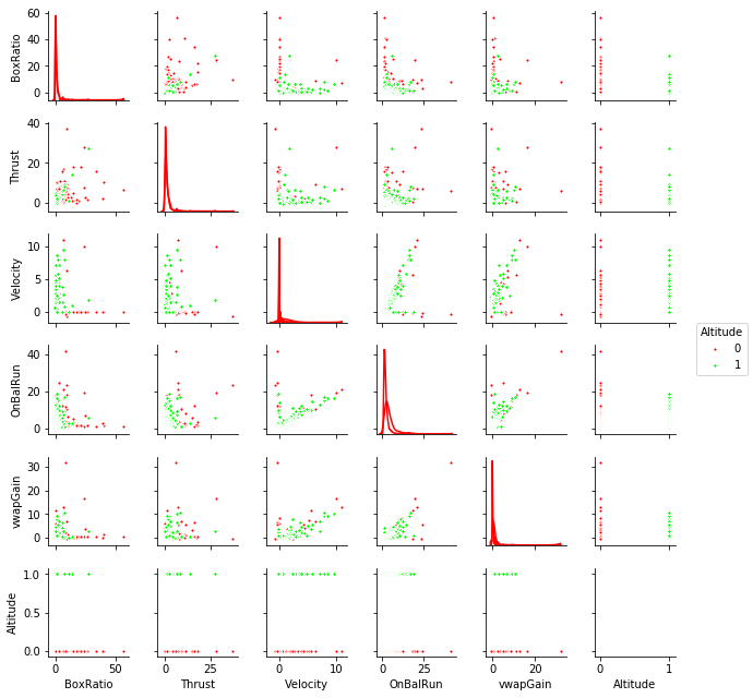
Get the training, validation, and testing datasets, and display a pairs plot
x_train, y_train, x_valid, y_valid, x_test, y_test, train, valid, test = Get_Model_Data()
train_:
    BoxRatio  Thrust  Velocity  OnBalRun  vwapGain  Altitude
0     0.166   0.166     0.317     0.455    -0.068         0
1    -0.031  -0.031     0.109     0.531     0.115         0
2    -0.186  -0.193     0.344     0.548     0.111         0
3     0.101   0.101     0.288     0.628     0.045         0
4     0.289   0.289     0.383     0.685     0.051         0
valid_:
    BoxRatio  Thrust  Velocity  OnBalRun  vwapGain  Altitude
0     0.071   0.068     0.170     0.482    -0.231         0
1    -0.147  -0.147     0.326     0.597     0.157         1
2     0.108   0.150    -0.005     0.823     0.599         0
3     0.634   0.550    -0.016     0.836     0.538         0
4     0.489   0.647    -0.012     0.838     0.393         0
test_:
    BoxRatio  Thrust  Velocity  OnBalRun  vwapGain  Altitude
0     0.023   0.023     0.182     0.711     0.131         1
1     0.912   1.449    -0.003     0.814     0.072         0
2     0.910  -0.030    -0.006     0.818     0.159         0
3     0.076   0.031    -0.003     0.829     0.090         0
4     1.237   1.457    -0.030     0.831     0.486         0
Define the hyper-parameters
hidden_list = list([[40],[80],[100],[200],[300],[400],[500],
                   [80,40],[100,50],[200,100],[300,150],[400,200], [500,250],
                   [80,70,60,50],
                   [100,80,60,40],
                   [200,150,100,50],
                   [300,250,200,150],
                   [80,70,60,50,40],
                   [100,80,60,40,20],
                   [200,180,160,140,120],
                   [300,250,200,150,100],
                   [400,350,300,250,200],
                   [500,400,300,200,100],
                   [80,70,60,50,40,30],
                   [100,90,80,70,60,50],
                   [200,180,160,150,140,130],
                   [300,250,200,150,100,50],
                   [400,350,300,250,200,150],
                   [500,400,300,200,100,50]])

activation_list = ['tanh', 'tanh_with_dropout', 'rectifier', 'rectifier_with_dropout', 'maxout']
best_mse = 100000.0
best_auc = 0.0
loop = 0
max_loop = 200
start_time = int(time.time())

space = {
    'hidden': hp.choice('hidden', hidden_list),
    'activation': hp.choice('activation', activation_list)
}
Now run the Bayesian search
trials = Trials()
Compute the metrics and display the results
best = fmin(objective, space, algo=tpe.suggest, max_evals=max_loop)
best_hidden = hidden_list[best['hidden']]
best_activation = activation_list[best['activation']]
print('\nbest model:',
'\n hidden........ ', best_hidden,
'\n activation.... ', best_activation,
'\n best mse...... ', best_mse,
'\n type.......... ', best_nn.type)
print('\nModel performance:')
performance = best_nn.model_performance(test_data = test)
print('\nPerformance: ', performance)
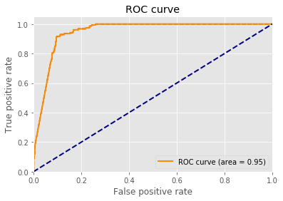
ROC_Curve(best_nn, train)
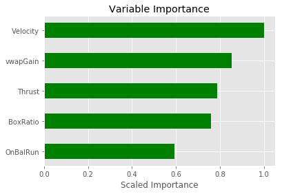
Plot_predictor_importance(best_nn)
test_actual = test.as_data_frame(use_pandas=True)['Altitude']
predicted = best_nn.predict(x_test).as_data_frame(use_pandas=True)
test_predicted = predicted['predict']
cm = metrics.confusion_matrix(test_actual, test_predicted)
performance_train = best_nn.model_performance(train)
auc = best_nn.auc()
Print_results(cm, auc, 'Model performance on training data')
1 hid: [500, 400, 300, 200, 100, 50] , act: maxout , best auc: 0.29494287191281504
2 hid: [300, 250, 200, 150, 100] , act: tanh , best auc: 0.8161596477670997
3 hid: [300] , act: rectifier , best auc: 0.8572061569624526
5 hid: [100, 50] , act: tanh , best auc: 0.8894864274636817
13 hid: [500, 250] , act: rectifier_with_dropout , best auc: 0.8996028009167453
22 hid: [500, 250] , act: rectifier_with_dropout , best auc: 0.9042273729519872
45 hid: [100, 50] , act: rectifier_with_dropout , best auc: 0.9078912549550898
50 , auc: 0.8125002476669771
72 hid: [500, 400, 300, 200, 100] , act: rectifier_with_dropout , best auc: 0.9112721153744711
100 , auc: 0.8916750873438873
145 hid: [500, 400, 300, 200, 100] , act: rectifier , best auc: 0.9275929188601812
146 hid: [500, 400, 300, 200, 100] , act: rectifier , best auc: 0.9305512019908126
150 , auc: 0.9279331553905071
153 hid: [500, 400, 300, 200, 100] , act: rectifier , best auc: 0.9473137334349484
200 , auc: 0.5

best model:
 hidden........  [500, 400, 300, 200, 100]
 activation....  rectifier
 best mse......  0.18319701560696858
 type..........  classifier

Model performance:

Performance:
ModelMetricsBinomial: deeplearning
** Reported on test data. **

MSE: 0.05304878563082557
RMSE: 0.23032321991242127
LogLoss: 0.2771598637210761
Mean Per-Class Error: 0.07693160403502941
AUC: 0.9202970845804235
Gini: 0.840594169160847
Confusion Matrix (Act/Pred) for max f1 @ threshold = 0.4531084961389309:
| 0 | 1 | Error | Rate | |
| 0 | 269.0 | 22.0 | 0.0756 | (22.0/291.0) |
| 1 | 4.0 | 27.0 | 0.129 | (4.0/31.0) |
| Total | 273.0 | 49.0 | 0.0807 | (26.0/322.0) |
Maximum Metrics: Maximum metrics at their respective thresholds
| metric | threshold | value | idx |
| max f1 | 0.4531085 | 0.6750000 | 6.0 |
| max f2 | 0.1660037 | 0.8100559 | 12.0 |
| max f0point5 | 0.4531085 | 0.5947137 | 6.0 |
| max accuracy | 0.4531085 | 0.9192547 | 6.0 |
| max precision | 0.9970580 | 1.0 | 0.0 |
| max recall | 0.0000000 | 1.0 | 260.0 |
| max specificity | 0.9970580 | 1.0 | 0.0 |
| max absolute_mcc | 0.1660037 | 0.6631793 | 12.0 |
| max min_per_class_accuracy | 0.1660037 | 0.9106529 | 12.0 |
| max mean_per_class_accuracy | 0.1660037 | 0.9230684 | 12.0 |
Gains/Lift Table: Avg response rate: 9.63 %
| group | cumulative_data_fraction | lower_threshold | lift | cumulative_lift | response_rate | cumulative_response_rate | capture_rate | cumulative_capture_rate | gain | cumulative_gain | |
| 1 | 0.0124224 | 0.5088962 | 5.1935484 | 5.1935484 | 0.5 | 0.5 | 0.0645161 | 0.0645161 | 419.3548387 | 419.3548387 | |
| 2 | 0.1459627 | 0.5068352 | 5.5558890 | 5.5250515 | 0.5348837 | 0.5319149 | 0.7419355 | 0.8064516 | 455.5888972 | 452.5051476 | |
| 3 | 0.1521739 | 0.4480430 | 10.3870968 | 5.7235023 | 1.0 | 0.5510204 | 0.0645161 | 0.8709677 | 938.7096774 | 472.3502304 | |
| 4 | 0.2018634 | 0.0066091 | 1.2983871 | 4.6342432 | 0.125 | 0.4461538 | 0.0645161 | 0.9354839 | 29.8387097 | 363.4243176 | |
| 5 | 0.3012422 | 0.0000560 | 0.0 | 3.1054207 | 0.0 | 0.2989691 | 0.0 | 0.9354839 | -100.0 | 210.5420685 | |
| 6 | 0.4006211 | 0.0000036 | 0.3245968 | 2.4156039 | 0.03125 | 0.2325581 | 0.0322581 | 0.9677419 | -67.5403226 | 141.5603901 | |
| 7 | 0.5 | 0.0000004 | 0.0 | 1.9354839 | 0.0 | 0.1863354 | 0.0 | 0.9677419 | -100.0 | 93.5483871 | |
| 8 | 0.5993789 | 0.0000000 | 0.0 | 1.6145746 | 0.0 | 0.1554404 | 0.0 | 0.9677419 | -100.0 | 61.4574628 | |
| 9 | 0.6987578 | 0.0000000 | 0.0 | 1.3849462 | 0.0 | 0.1333333 | 0.0 | 0.9677419 | -100.0 | 38.4946237 | |
| 10 | 0.7981366 | 0.0000000 | 0.0 | 1.2125016 | 0.0 | 0.1167315 | 0.0 | 0.9677419 | -100.0 | 21.2501569 | |
| 11 | 0.8975155 | 0.0000000 | 0.0 | 1.0782453 | 0.0 | 0.1038062 | 0.0 | 0.9677419 | -100.0 | 7.8245340 | |
| 12 | 1.0 | 0.0000000 | 0.3147605 | 1.0 | 0.0303030 | 0.0962733 | 0.0322581 | 1.0 | -68.5239492 | 0.0 |
Confusion matrix:
 [[261  30]
 [  2  29]]

Model performance on training data
misclassification_rate... 0.0994
accuracy................. 0.9006
precision................ 0.4915
recall................... 0.9355
F1....................... 0.6444
auc...................... 0.9473

Computed another way:
Correct classifications on all data: 290/322 (90.062112)
accuracy................. 0.900621118012
precision................ 0.491525423729
recall................... 0.935483870968
F1....................... 0.644444444444
Save the model
model_path = h2o.save_model(model=best_nn, path="C:/sm/BottleRockets/trained_models/h2o_nn_classify", force=True)
Load the trained model and print the results
# load the model
saved_nn = h2o.load_model(model_path)

print('\nMetrics summary:\n', saved_nn.cross_validation_metrics_summary())

Print_Metrics(saved_nn)
Metrics summary:
 Cross-Validation Metrics Summary:
| mean | sd | cv_1_valid | cv_2_valid | cv_3_valid | cv_4_valid | cv_5_valid | |
| accuracy | 0.5827555 | 0.2627193 | 0.9070632 | 0.1232394 | 0.1330935 | 0.8571429 | 0.8932384 |
| auc | 0.7180123 | 0.1243454 | 0.8909345 | 0.5 | 0.5135135 | 0.8887383 | 0.796875 |
| err | 0.4172445 | 0.2627193 | 0.0929368 | 0.8767605 | 0.8669065 | 0.1428571 | 0.1067616 |
| err_count | 116.8 | 74.10587 | 25.0 | 249.0 | 241.0 | 39.0 | 30.0 |
| f0point5 | 0.3629290 | 0.1256493 | 0.5963303 | 0.1494449 | 0.1610096 | 0.4382470 | 0.4696132 |
| f1 | 0.4382103 | 0.1274818 | 0.6753247 | 0.2194357 | 0.2349206 | 0.5301205 | 0.53125 |
| f2 | 0.5815387 | 0.0988973 | 0.7784431 | 0.4127359 | 0.4342723 | 0.6707317 | 0.6115108 |
| lift_top_group | 3.8473048 | 2.0918105 | 8.966666 | 1.0 | 1.0 | 3.3703704 | 4.899487 |
| logloss | 0.5046766 | 0.2165145 | 0.2345611 | 0.3744118 | 1.0471588 | 0.6265903 | 0.2406613 |
| max_per_class_error | 0.5277037 | 0.2760644 | 0.1333333 | 1.0 | 1.0 | 0.1851852 | 0.32 |
| mcc | 0.545003 | 0.0617232 | 0.6455954 | NaN | NaN | 0.5002185 | 0.4891951 |
| mean_per_class_accuracy | 0.7049466 | 0.1201218 | 0.8894003 | 0.5 | 0.5 | 0.8383017 | 0.7970312 |
| mean_per_class_error | 0.2950534 | 0.1201218 | 0.1105997 | 0.5 | 0.5 | 0.1616983 | 0.2029688 |
| mse | 0.1500674 | 0.0955273 | 0.0627303 | 0.1083020 | 0.4179803 | 0.0960079 | 0.0653165 |
| precision | 0.3276558 | 0.1210266 | 0.5531915 | 0.1232394 | 0.1330935 | 0.3928571 | 0.4358974 |
| r2 | -0.4282405 | 0.7835595 | 0.3669136 | -0.0023190 | -2.6226525 | -0.0772917 | 0.1941471 |
| recall | 0.8722963 | 0.0853991 | 0.8666667 | 1.0 | 1.0 | 0.8148148 | 0.68 |
| rmse | 0.3582979 | 0.1041395 | 0.2504602 | 0.3290928 | 0.646514 | 0.3098514 | 0.2555710 |
| specificity | 0.537597 | 0.3106647 | 0.9121339 | 0.0 | 0.0 | 0.8617886 | 0.9140625 |
Model performance on validate and test data set:
Percent correct predictions on test set (accuracy):  0.900621118012
| Metric | Validate | Test |
| logloss | 0.6237310 | 0.2771599 |
| accuracy | 0.8836478 | 0.9192547 |
| precision | 1.0 | 1.0 |
| F1 | 0.6226415 | 0.6750000 |
| r2 | 0.2773331 | 0.3902771 |
| AUC | 0.8461331 | 0.9202971 |
Print the total elapsed computation time, and shut down the server
end_time = int(time.time())
d = divmod(end_time - start_time,86400)  # days
h = divmod(d[1],3600)  # hours
m = divmod(h[1],60)  # minutes
s = m[1]  # seconds
print('%d days, %d hours, %d minutes, %d seconds' % (d[0],h[0],m[0],s))

h2o.cluster().shutdown()
0 days, 6 hours, 31 minutes, 54 seconds
H2O session _sid_84ba closed.
Discussion
The H2O Neural Network has performed well, considering it’s out first attempt. You will notice that the Variable Importance’s is much better for the neural network than the Random Forest model. The auc is better for the Neural Network model than the Random Forest model.