H2o Automl
Analyze the Bottle Rocket dataset using H2O AutoML
This is our second generation model. The models for the first generation analysis were summarized on October 17, 2017. A lot has happened since then. This analysis was done on August 2, 2018. We have achieved a major improvement in the results. Please see the Summary below.
import platform, time, sys
import numpy as np
import pandas as pd
import matplotlib
from matplotlib import pyplot as plt
%matplotlib inline
import itertools
from imblearn.over_sampling import SMOTE
from tabulate import tabulate
import seaborn as sns

from sklearn.metrics import accuracy_score, auc, classification_report, confusion_matrix, f1_score
from sklearn.metrics import log_loss, mean_squared_error, precision_score, recall_score, r2_score
from sklearn.metrics import roc_auc_score, roc_curve
from sklearn.model_selection import train_test_split

import h2o
from h2o.automl import H2OAutoML
import warnings
warnings.filterwarnings("ignore")
print('Operating system version....', platform.platform())
print("Python version is........... %s.%s.%s" % sys.version_info[:3])
print('pandas version is...........', pd.__version__)
print('numpy version is............', np.__version__)
print('matplotlib version is.......', matplotlib.__version__)
Operating system version.... Windows-10-10.0.17134-SP0
Python version is........... 3.6.5
pandas version is........... 0.23.0
numpy version is............ 1.14.3
matplotlib version is....... 2.2.2
Start the h2o server
start_time = int(time.time())

localH2O = h2o.init(ip = "localhost",
                    port = 54321,
                    max_mem_size="24G",
                    nthreads = 6)
h2o.no_progress()
h2o.remove_all()
Checking whether there is an H2O instance running at http://localhost:54321..... not found.
Attempting to start a local H2O server...
  Java HotSpot(TM) 64-Bit Server VM (build 25.181-b13, mixed mode)
  Starting server from C:\Users\Charles\Anaconda3\lib\site-packages\h2o\backend\bin\h2o.jar
  Ice root: C:\Users\Charles\AppData\Local\Temp\tmpawu4yul2
  JVM stdout: C:\Users\Charles\AppData\Local\Temp\tmpawu4yul2\h2o_Charles_started_from_python.out
  JVM stderr: C:\Users\Charles\AppData\Local\Temp\tmpawu4yul2\h2o_Charles_started_from_python.err
  Server is running at http://127.0.0.1:54321
Connecting to H2O server at http://127.0.0.1:54321... successful.

H2O cluster timezone:
H2O cluster version: 3.21.0.4374
H2O cluster version age: 3 days
H2O cluster name: H2O_from_python_Charles
H2O cluster total nodes: 1
H2O cluster free memory: 21.33 Gb
H2O cluster total cores: 0
H2O cluster allowed cores: 0
H2O cluster status: accepting new members, healthy
H2O connection url: http://127.0.0.1:54321
H2O connection proxy: None
H2O internal security: False
H2O API Extensions: Algos, AutoML, Core V3, Core V4
Python version: 3.6.5 final
Define a correlation plot
def Correlation_plot(df_new, response_column):
    plt.ioff()
    red_green = ["#ff0000", "#00ff00"]
    sns.set_palette(red_green)
    np.seterr(divide='ignore', invalid='ignore')
    g = sns.pairplot(df_new,
                     diag_kind='kde',
                     hue=response_column,
                     markers=["o", "D"],
                     size=1.5,
                     aspect=1,
                     plot_kws={"s": 10})
    g.fig.subplots_adjust(right=0.9)
    plt.show()
Define a method to get the data set, and split it into train, validate, test
def Get_Model_Data():
    path = 'https://raw.githubusercontent.com/CBrauer/CypressPoint.github.io/master/model-13-1.csv'
    model = pd.read_csv(path)

    feature_columns = ['BoxRatio','Thrust', 'Velocity', 'OnBalRun', 'vwapGain']
    response_column = ['Altitude']
    mask = feature_columns + response_column

    # Correlation_plot(model[mask], response_column)

    X = model[feature_columns].values
    y = model[response_column].values.ravel()

    sm = SMOTE(random_state=12)
    X_resampled, y_resampled = sm.fit_sample(X, y)

    X_train, X_test, y_train, y_test = train_test_split(X_resampled,
                                                        y_resampled,
                                                        test_size = 0.3,
                                                        random_state = 0)
    # reshape so we can append the columns
    y_train_ = y_train.reshape(y_train.shape[0], 1)
    df_train = pd.DataFrame(X_train, columns=feature_columns)
    df_train[response_column] = pd.DataFrame(y_train_).astype(int)
    print('train: \n', df_train.head(5))

    y_test_ = y_test.reshape(y_test.shape[0], 1)
    df_test = pd.DataFrame(X_test, columns=feature_columns)
    df_test[response_column] = pd.DataFrame(y_test_).astype(int)
    print('test: \n',  df_test.head(5))

    train = h2o.H2OFrame(df_train)
    train[response_column] = train[response_column].asfactor()
    X_train = train[feature_columns]
    y_train = train[response_column]

    test = h2o.H2OFrame(df_test)
    test[response_column] = test[response_column].asfactor()
    X_test = test[feature_columns]
    y_test = test[response_column]

    return X_train, y_train, X_test, y_test, train, test, feature_columns, response_column
Plot the ROC curve
def ROC_Curve(best_model, train):
    performance = best_model.model_performance(train)
    auc = performance.auc()
    false_positive_rate = performance.fprs
    true_positive_rate = performance.tprs

    plt.style.use('ggplot')
    plt.figure()
    plt.plot(false_positive_rate, true_positive_rate, 'k--')
    plt.plot(false_positive_rate,
             true_positive_rate,
             color='darkorange',
             lw = 2,
             label='ROC curve (area = %0.2f)' % auc)
    plt.plot([0,1], [0,1], color = 'navy', lw = 2, linestyle = '--')
    plt.xlim(0, 0.2)
    plt.ylim(0.8, 1)
    plt.xlabel('False positive rate')
    plt.ylabel('True positive rate')
    plt.title('ROC curve')
    plt.legend(loc='best')
    plt.show()
Plot the performance of each predictor
def Plot_predictor_importance(best_model):
    fig, ax = plt.subplots()
    variables = best_model._model_json['output']['variable_importances']['variable']
    y_pos = np.arange(len(variables))
    scaled_importance = best_model._model_json['output']['variable_importances']['scaled_importance']
    ax.barh(y_pos,
            scaled_importance,
            align='center',
            color='green',
            ecolor='black',
            height=0.5)
    ax.set_yticks(y_pos)
    ax.set_yticklabels(variables)
    ax.invert_yaxis()
    ax.set_xlabel('Scaled Importance')
    ax.set_title('Variable Importance')
    plt.show()
Plot the confusion matrix
def Plot_Confusion_Matrix(best_model):
    y_predicted = best_model.predict(X_test)
    y_predicted_ = y_predicted.as_data_frame(use_pandas=True, header=False)
    y_pred = y_predicted_['predict']

    y_test_ = y_test.as_data_frame(use_pandas=True, header=False)
    y = y_test_[response_column]

    cm = confusion_matrix(y, y_pred)

    cmap = plt.cm.Blues
    plt.imshow(cm, interpolation='nearest', cmap=cmap)
    title='Confusion matrix (on test data)'
    classes = [0, 1]
    plt.title(title)
    plt.colorbar()
    tick_marks = np.arange(len(classes))
    plt.xticks(tick_marks, classes, rotation=0)
    plt.yticks(tick_marks, classes)

    thresh = cm.max() / 2.
    for i, j in itertools.product(range(cm.shape[0]), range(cm.shape[1])):
        plt.text(j, i, cm[i, j],
                 horizontalalignment="center",
                 color="white" if cm[i, j] > thresh else "black")
    plt.tight_layout()
    plt.ylabel('True label')
    plt.xlabel('Predicted label')

    c_report = classification_report(y, y_pred)
    print('\nClassification report:\n', c_report)
Print the model metrics for the validate and test data sets
def Print_Metrics(best_model, X_test, y_test):
    print('\nModel performance on test data set:')

    predictions = best_model.predict(X_test)
    misclassification_rate = (predictions['predict'] == y_test).as_data_frame(use_pandas=True).mean()

    performance = best_model.model_performance(test)
    accuracy  = performance.accuracy()[0][1]
    precision = performance.precision()[0][1]
    recall    = 0.0  #performance.recall()[0][1]  not available yet
    F1        = performance.F1()[0][1]
    r2        = performance.r2()
    auc       = performance.auc()
    mse       = performance.mse()
    logloss   = performance.logloss()

    header = ["Metric", "Test dataset"]
    table = [["accuracy",               accuracy],
             ["precision",              precision],
             ["recall",                 recall],
             ["misclassification rate", misclassification_rate],
             ["F1",                     F1],
             ["r2",                     r2],
             ["AUC",                    auc],
             ["mse",                    mse],
             ["logloss",                logloss]
            ]

    print(tabulate(table, header, tablefmt="fancy_grid", floatfmt=".8f"))
Load the Bottle Rocket dataset
X_train, y_train, X_test, y_test, train, test, feature_columns, response_column = Get_Model_Data()
train:
    BoxRatio    Thrust  Velocity  OnBalRun  vwapGain  Altitude
0  0.324000  0.615000  1.525000  3.618000  0.416000         0
1  0.938249  0.366377  2.402230  6.393223  2.667106         1
2  0.317000 -0.281000  0.979000  1.489000  0.506000         0
3  0.289000 -0.433000  0.796000  2.081000  0.536000         0
4  1.551115 -0.103734  0.731682  1.752156  0.667016         1
test:
    BoxRatio    Thrust  Velocity  OnBalRun  vwapGain  Altitude
0  0.051000 -0.419000  0.351000  1.173000  0.571000         0
1  3.832137  0.933219  0.918407  3.290789  0.501965         1
2  1.252387  2.489781  1.461396  4.268061  1.055923         1
3  0.000000 -0.814201  0.883223  1.960900  0.269550         1
4  0.222000 -0.296000  1.057000  2.714000  0.808000         0
Define the AutoML model.
def Run():
    aml = H2OAutoML(max_models = 500,
                    seed = 7,
                    max_runtime_secs = 1*60*60,
                    nfolds = 5,
                    stopping_metric = "misclassification",
                    project_name="bottle_rocket",
                    stopping_rounds = 5)

    aml.train(x = feature_columns,
              y = 'Altitude',
              training_frame = train)

    lb = aml.leaderboard
    return lb, X_test, y_test, train, test, feature_columns, response_column
Now let’s run the model and get the best model from the leaderboard
lb = Run()
Choose the best model from the leader board.
At this time, we cannot choose a Stacked Ensemble model because it lacks the metrics we want.
df = lb[0][0]
print('df:\n', df)
df2 = df.as_data_frame(use_pandas=True, header=True)

for row in range(len(lb)):
    model_id = df2.iloc[row,0]
    print('model_id:', model_id)
    if 'StackedEnsemble' in model_id:
        continue
    else:
        best_model = h2o.get_model(model_id)
        break
df:
| model_id |
|---|
| StackedEnsemble_AllModels_0_AutoML_20180804_081525 |
| GBM_grid_0_AutoML_20180804_081525_model_21 |
| GBM_grid_0_AutoML_20180804_081525_model_63 |
| StackedEnsemble_AllModels_0_AutoML_20180804_071054 |
| StackedEnsemble_BestOfFamily_0_AutoML_20180804_071054 |
| GBM_grid_0_AutoML_20180804_081525_model_291 |
| DRF_0_AutoML_20180804_071054 |
| DRF_0_AutoML_20180804_081525 |
| GBM_grid_0_AutoML_20180804_081525_model_20 |
| XRT_0_AutoML_20180804_081525 |
model_id: StackedEnsemble_AllModels_0_AutoML_20180804_081525
model_id: GBM_grid_0_AutoML_20180804_081525_model_21
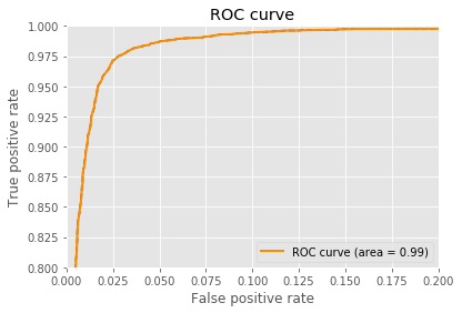
Plot the ROC Curve
ROC_Curve(best_model, train)
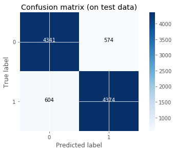
Plot the confusion matrix
Plot_Confusion_Matrix(best_model)
Classification report:
              precision    recall  f1-score   support

          0       0.88      0.88      0.88      4915
          1       0.88      0.88      0.88      4978

avg / total       0.88      0.88      0.88      9893
Save the model
model_path = h2o.save_model(model=best_model, path="C:/sm/trained_models/h2o_automl", force=True)
Load the model
saved_model = h2o.load_model(model_path)
Plot predictor importance
Plot_predictor_importance(saved_model)

Print the performance of the model
Note that ‘recall’ is not available in this version of h2o.automl
Print_Metrics(saved_model, X_test, y_test)
Model performance on test data set:
╒════════════════════════╤════════════════╕
│ Metric                 │   Test dataset │
╞════════════════════════╪════════════════╡
│ accuracy               │     0.88314970 │
├────────────────────────┼────────────────┤
│ precision              │     1.00000000 │
├────────────────────────┼────────────────┤
│ recall                 │     0.00000000 │
├────────────────────────┼────────────────┤
│ misclassification rate │     0.88092591 │
├────────────────────────┼────────────────┤
│ F1                     │     0.88748788 │
├────────────────────────┼────────────────┤
│ r2                     │     0.61682860 │
├────────────────────────┼────────────────┤
│ AUC                    │     0.95078805 │
├────────────────────────┼────────────────┤
│ mse                    │     0.09578897 │
├────────────────────────┼────────────────┤
│ logloss                │     0.32046170 │
╘════════════════════════╧════════════════╛
Print the computation time
end_time = int(time.time())
d = divmod(end_time - start_time,86400)  # days
h = divmod(d[1],3600)  # hours
m = divmod(h[1],60)  # minutes
s = m[1]  # seconds
print('%d days, %d hours, %d minutes, %d seconds' % (d[0],h[0],m[0],s))
0 days, 0 hours, 15 minutes, 58 seconds