Automl Sklearn
Analysis of the Bottle Rocket pattern in the stock market
This is our second generation model. The models for the first generation analysis were summarized on October 17, 2017. This analysis was done on August 3, 2018. We have achieved a major improvement in the results by using autoML. Please see the Summary below.
import sklearn.model_selection
from sklearn.metrics import roc_auc_score, roc_curve, auc, classification_report
from sklearn.metrics import confusion_matrix, accuracy_score, mean_squared_error
from sklearn.metrics import f1_score, r2_score, precision_score, recall_score
from sklearn.metrics import log_loss
from sklearn.model_selection import train_test_split
from sklearn.metrics import confusion_matrix
from sklearn.externals import joblib

import pandas as pd
import numpy as np
import itertools
from imblearn.over_sampling import SMOTE
from tabulate import tabulate
from matplotlib import pyplot as plt
%matplotlib inline
import time

import autosklearn.classification
from autosklearn.metrics import accuracy, f1_macro, roc_auc

import warnings
warnings.filterwarnings("ignore")
The LoadData routine is used to read the Bottle Rocket dataset, and create training and testing datasets
def LoadData():
    global feature_names, response_name, n_features

    model_full = pd.read_csv('https://raw.githubusercontent.com/CBrauer/CypressPoint.github.io/master/model-13-1.csv')

    response_name = ['Altitude']
    feature_names = ['BoxRatio', 'Thrust', 'Velocity', 'OnBalRun', 'vwapGain']
    n_features = len(feature_names)
    mask = feature_names + response_name

    model = model_full[mask]
    print('Model dataset:\n', model.head(5))
    # print('\nDescription of model dataset:\n', model[feature_names].describe(include='all'))

    # Correlation_plot(model)

    X = model[feature_names].values
    y = model[response_name].values.ravel()

    sm = SMOTE(random_state=12)
    X_resampled, y_resampled = sm.fit_sample(X, y)

    X_train, X_test, y_train, y_test = train_test_split(X_resampled,
                                                        y_resampled,
                                                        test_size = 0.3,
                                                        random_state = 0)
    print('Size of resampled data:')
    print(' train shape... ', X_train.shape, y_train.shape)
    print(' test shape.... ', X_test.shape, y_test.shape)

    return X_train, y_train, X_test, y_test
This routine is used to summarize the metrics for the model.
def Print_model_metrics():
    true_negative_test  = cm_test[0, 0]
    true_positive_test  = cm_test[1, 1]
    false_negative_test = cm_test[1, 0]
    false_positive_test = cm_test[0, 1]
    total_test = true_negative_test + true_positive_test + false_negative_test + false_positive_test
    accuracy_test = (true_positive_test + true_negative_test)/total_test
    misclassification_rate_test = (false_positive_test + false_negative_test)/total_test
    mse_test       = mean_squared_error(y_test, y_predict_test)
    logloss_test   = log_loss(y_test, y_predict_test)
    accuracy_test  = accuracy_score(y_test, y_predict_test)
    precision_test = precision_score(y_test, y_predict_test, average='binary')
    recall_test    = recall_score(y_test, y_predict_test, average='binary')
    F1_test        = f1_score(y_test, y_predict_test)
    r2_test        = r2_score(y_test, y_predict_test)
    auc_test       = roc_auc_score(y_test, y_predict_test)

    header = ["Metric", "auto-sklearn"]
    table = [["accuracy",               accuracy_test],
             ["precision",              precision_test],
             ["recall",                 recall_test],
             ["misclassification rate", misclassification_rate_test],
             ["F1",                     F1_test],
             ["r2",                     r2_test],
             ["AUC",                    auc_test],
             ["mse",                    mse_test],
             ["logloss",                logloss_test]
            ]

    print(tabulate(table, header, tablefmt="fancy_grid", floatfmt=".8f"))
Now let’s load the data
start_time = int(time.time())

X_train, y_train, X_test, y_test = LoadData()
Model dataset:
    BoxRatio   Thrust  Velocity  OnBalRun  vwapGain  Altitude
0     0.831   -0.076     0.381     1.006     0.444         0
1     0.497    0.333     0.489     1.453     0.411         0
2     0.667   -0.127     0.740     2.157     0.455         0
3     0.171   -0.428     0.454     0.940     0.451         0
4   265.390  183.215     8.967    29.467    20.560         0
Size of resampled data:
 train shape...  (23083, 5) (23083,)
 test shape....  (9893, 5) (9893,)
The ROC_Curve routine is used to plot the ROC curve.
def ROC_Curve():
    plt.figure()
    plt.plot([0, 1], [0, 1], 'k--')
    plt.plot(false_positive_rate, true_positive_rate, color='darkorange', label='Random Forest')
    plt.xlabel('False positive rate')
    plt.ylabel('True positive rate')
    plt.title('ROC curve (area = %0.7f)' % auc)
    plt.legend(loc='best')
    plt.show()
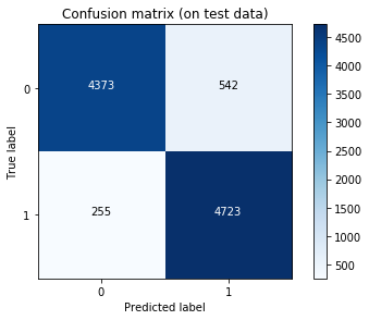
This routine plots the confusion matrix.
def Plot_confusion_matrix():
    cm_test = confusion_matrix(y_test, y_predict_test)
    cmap = plt.cm.Blues
    plt.imshow(cm_test, interpolation='nearest', cmap=cmap)
    title='Confusion matrix (on test data)'
    classes = [0, 1]
    plt.title(title)
    plt.colorbar()
    tick_marks = np.arange(len(classes))
    plt.xticks(tick_marks, classes, rotation=0)
    plt.yticks(tick_marks, classes)

    thresh = cm_test.max() / 2.
    for i, j in itertools.product(range(cm_test.shape[0]), range(cm_test.shape[1])):
        plt.text(j, i, cm_test[i, j],
                 horizontalalignment="center",
                 color="white" if cm_test[i, j] > thresh else "black")

    plt.tight_layout()
    plt.ylabel('True label')
    plt.xlabel('Predicted label')

    c_report = classification_report(y_test, y_predict_test)
    print('\nClassification report:\n', c_report)

    ntotal = len(y_test)
    correct = y_test == y_predict_test
    numCorrect = sum(correct)
    percent = round( (100.0*numCorrect)/ntotal, 6)
    print("\nCorrect classifications on test data: {0:d}/{1:d} {2:8.3f}%".format(numCorrect,
                                                                                 ntotal,
                                                                                 percent))
    return cm_test
Define how we are going to run the model.
def Run_model():
    automl = autosklearn.classification.AutoSklearnClassifier(time_left_for_this_task=36000)
    automl.fit(X_train, y_train, dataset_name='bottle_rocket')
    automl.fit_ensemble(y_train, ensemble_size=50, metric=roc_auc)
    y_predict_test = automl.predict(X_test)
    return automl, y_predict_test
Now, run the model.
automl, y_predict_test = Run_model()
[WARNING] [2018-06-22 17:20:30,032:EnsembleBuilder(1):bottle_rocket] No models better than random - using Dummy Classifier!
[WARNING] [2018-06-22 17:20:30,066:EnsembleBuilder(1):bottle_rocket] No models better than random - using Dummy Classifier!
[WARNING] [2018-06-22 17:20:32,071:EnsembleBuilder(1):bottle_rocket] No models better than random - using Dummy Classifier!
[WARNING] [2018-06-22 17:20:34,076:EnsembleBuilder(1):bottle_rocket] No models better than random - using Dummy Classifier!
[WARNING] [2018-06-22 17:21:47,957:smac.intensification.intensification.Intensifier] Challenger was the same as the current incumbent; Skipping challenger
[WARNING] [2018-06-22 17:21:47,957:smac.intensification.intensification.Intensifier] Challenger was the same as the current incumbent; Skipping challenger
Print the score of the test dataset, and save the model to our disk.
# Show the final ensemble produced by Auto-sklearn.
# print('\nModels: \n', automl.show_models())
print('\nStatistics: \n', automl.sprint_statistics())
# Show the actual model scores and the hyperparameters used. \
# print('\ncv results: \n', automl.cv_results_)
score = accuracy_score(y_test, y_predict_test)
name = automl._automl._metric.name
print("\nAccuracy score {0:.8f} using {1:s}".format(score, name))

joblib.dump(automl, 'automl.pkl')
Statistics:
 auto-sklearn results:
  Dataset name: bottle_rocket
  Metric: roc_auc
  Best validation score: 0.904699
  Number of target algorithm runs: 462
  Number of successful target algorithm runs: 429
  Number of crashed target algorithm runs: 3
  Number of target algorithms that exceeded the time limit: 30
  Number of target algorithms that exceeded the memory limit: 0


Accuracy score 0.91943799 using roc_auc


['automl.pkl']
Plot the confusion matrix.
cm_test = Plot_confusion_matrix()
Classification report:
              precision    recall  f1-score   support

          0       0.94      0.89      0.92      4915
          1       0.90      0.95      0.92      4978

avg / total       0.92      0.92      0.92      9893


Correct classifications on test data: 9096/9893   91.944%
Plot the ROC curve.
# Since our target is (0,1), the classifier produces a probability matrix of (N,2).
# The first column refers to the probability that our data belong to class 0 (failure to reach altitude),
# and the second column refers to the probability that the data belong to class 1 (it's a bottle rocket).
# Therefore, let's take the second column to compute the 'auc' metric.
y_probabilities_test = automl.predict_proba(X_test)
y_probabilities_success = y_probabilities_test[:, 1]

false_positive_rate, true_positive_rate, threshold = roc_curve(y_test, y_probabilities_success)
y_predicted_train = automl.predict(X_train)
auc = roc_auc_score(y_train, y_predicted_train)
ROC_Curve()

Print some metrics on the test dataset.
Print_model_metrics()
╒════════════════════════╤════════════════╕
│ Metric                 │   auto-sklearn │
╞════════════════════════╪════════════════╡
│ accuracy               │     0.91943799 │
├────────────────────────┼────────────────┤
│ precision              │     0.89705603 │
├────────────────────────┼────────────────┤
│ recall                 │     0.94877461 │
├────────────────────────┼────────────────┤
│ misclassification rate │     0.08056201 │
├────────────────────────┼────────────────┤
│ F1                     │     0.92219076 │
├────────────────────────┼────────────────┤
│ r2                     │     0.67773888 │
├────────────────────────┼────────────────┤
│ AUC                    │     0.91924997 │
├────────────────────────┼────────────────┤
│ mse                    │     0.08056201 │
├────────────────────────┼────────────────┤
│ logloss                │     2.78255718 │
╘════════════════════════╧════════════════╛
end_time = int(time.time())
d = divmod(end_time - start_time,86400)  # days
h = divmod(d[1],3600)  # hours
m = divmod(h[1],60)  # minutes
s = m[1]  # seconds
print('This analysis took: %d days, %d hours, %d minutes, %d seconds' % (d[0],h[0],m[0],s))
This analysis took: 0 days, 10 hours, 0 minutes, 49 seconds
Summary
The major improvements over the previous generation are a result of implementing:
- SMOTE. Dr. Jason Brownlee suggested that we use SMOTE click here to balance the dataset (it’s 13:1).
- auto-sklearn. Auto-sklearn is an automated machine learning toolkit and a drop-in replacement for a scikit-learn estimator click here
This jupyter notebook was run on bash, version 4.3.48(1)-release (x86_64-pc-linux-gnu). This Unix Shell is running on Ubuntu 16.04.4 LTS, under Windows 10 enterprise, release 17134.112.