
Figure 1. Start of the Bottle Rocket pattern
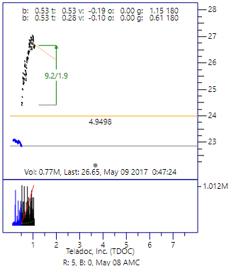
Figure 2. End of the Bottle Rocket pattern
Abstract - This is a case study on the use of machine learning to find the beginning of what we call the Bottle Rocket pattern in the stock market.
Keywords - machine learning, pattern recognition, stock market.
An interesting day-trading pattern is observed in the stock market. We call it the Bottle-Rocket Pattern. The easiest way to describe the pattern is with an example. Figures 1 and 2 show charts of Teladoc, Inc. (TDOC) that traded on May 9, 2017. The chart on the left shows the trade data at the point that the pattern was classified as the launch of a bottle rocket. The chart on the right shows the trading pattern about 40 minutes later. At this point, the algorithm had detected that the trajectory had topped-out, and the pattern was complete.
In this case study we analyze various Machine Learning packages to classify (recognize) the start of the pattern. The study is written from the point of view of a user of machine learning packages, not as a developer of a package.
|
Figure 1. Start of the Bottle Rocket pattern |
Figure 2. End of the Bottle Rocket pattern |
Please play the following video to see how a typical Bottle Rocket pattern develops:
Four Machine Learning packages were used to find the starting conditions of the Pattern.
The database, from which the training and testing datasets were derived, contains all the stocks on the major exchanges that have the following:
There are about 2,000 stocks in the database that meet this criterion, and the database is currently about 240 Giga-bytes.
The database starts on November 9, 2016 and continues to the present. The database contains all trades (summarized to 10 second intervals) for all the stocks that meet the minimum requirement, as well as day summaries (volume, open, high low, close). The trade data is captured in real-time from the IQFeed.net data service.
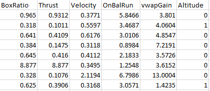
As new 10-second interval data comes in, five predictors (also known as “features”) are computed. The training and testing datasets consist of these predictor columns, plus a response variable column (actual outcome, a.k.a. ground-truth). Since we are doing “binary classification”, the response column (labeled “Altitude”) contains “1” for a successful pattern (the rocket proceeded upward for another 2%), and “0” for a pattern that failed (the rocket fizzled out). The first 8 rows of the training dataset are:
 |
|
Table 1. Dataframe format |
We clean the data at the end of the market each day with a custom computer program. Outliers are removed before the trade data is stored in the master database. Therefore, it is not necessary to do any outlier removal by a Machine learning algorithm.
The Candidate Filter is used to weed-out patterns that are obviously not candidates for further analysis. We do this because the machine classification step is very compute intensive. We analyze about 2,000 stocks per day. Even though the trades come into the computer at a near real-time rate, we need a filter to quickly reject the stock for further analysis. Hence, the candidate filter is used.
There are five components to the filter, and each one is based on common sense. For example, if the volume is too low, or the price is falling, it is obviously not a candidate for further analysis. If all five of the filter components meet a minimum criterion, then the machine classification computation begins. If the start of a Bottle Rocket pattern is recognized, an alert is given in the form of a chart like Figure 1.
The design and implementation of the Predictor filter is very simple (and hence fast). Also, the filter must be course enough to not filter out a desirable pattern. This, of course, will result in letting a lot of bad patterns through the filter. This results in a training dataset that is out-of-balance by about a factor of 13.
Speed is everything. In all the models, the processing time is much worse than one second. The average is about 3.5 seconds! This puts extra importance on the accuracy of the prediction.
We propose using the components of the Candidate filter as features of the Bottle Rocket dataset.
Now, we will discuss the five components of the Candidate filter.
The BoxRatio predictor is like the Equivolume box ratio that was developed by Mr. Richard W. Arms, Jr. of Albuquerque, New Mexico. Click here for more information.
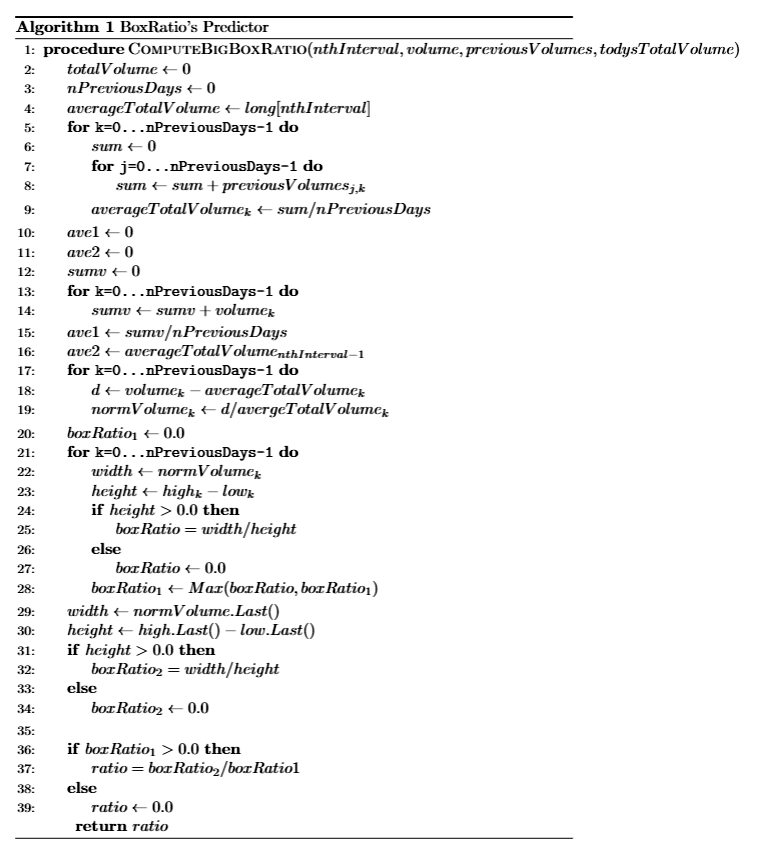
Here is the pseudocode that describes the BoxRatio algorithm.
|
The amount of fuel burning in a Bottle Rocket is analogous to the trading volume of a stock. This is best illustrated by the chart shown in Figure 3. The red line is the trading volume today that is summarized in 10-second intervals leading up to the classification of the pattern. There are 10 gray lines shown on the chart. These are the volume summaries for the preceding 10 days. The black line is the average of the 10 previous volume summaries.
The Thrust predictor is defined in algorithm 2.

|
The Thrust predictor is the percentage increase in today's volume, relative to the envelope formed by the previous 10 days. This computation is shown in the following pseudocode.
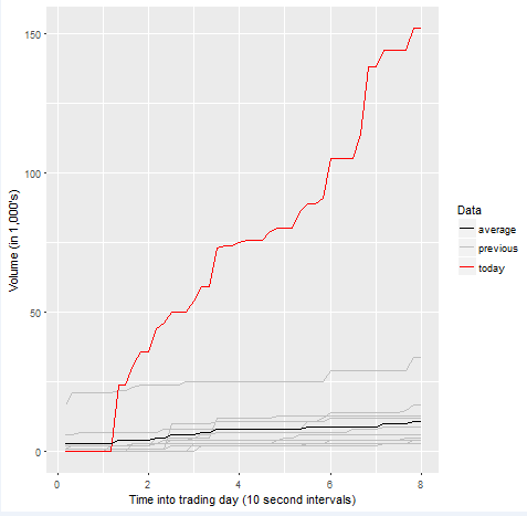
Figure 3 The Thrust predictor |
The data in Figure 3 starts at 48 intervals into the market. This clearly show that today’s volume is a significant increase over the volume in the proceeding previous ten days.
The Velocity predictor is the slope of the line through the proceeding 60 intervals. Algorithm 3 shows both the regression and velocity pseudocodes.

|
We define the velocity to be the slope of the linear regression that is fitted to the percentage change in the price data (blue dots). The regression line is shown in red in Figure 4.
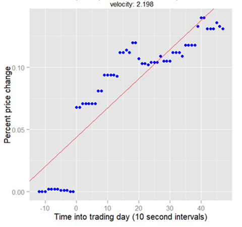
Figure 4 The Velocity predictor |
This predictor is called "OnBalRun". Shown in Figure 5.4.1 is the pseudocode for the computation of this predictor.
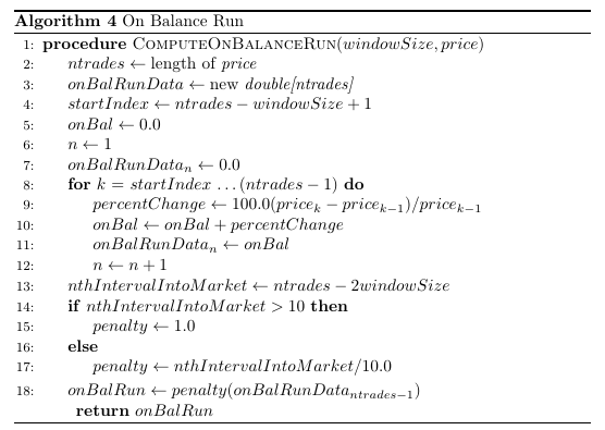
Figure 5.4.1 The OnBalRun predictor Pseudocode |
The blue dots on Figure 5.4.2 are the running total of the percent changes in the price. The value of the OnBalRun is the value of the last blue dot on the chart.
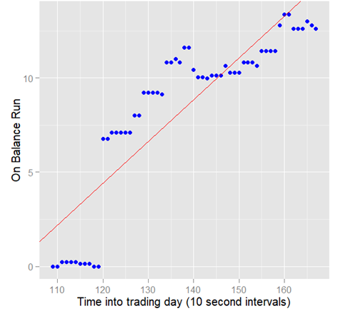
Figure 5.4.2 The OnBalRun predictor |
This predictor is based on a modified version of the Volume Weighted Average Price curve (VWAP). Shown in Figure 5.5.1 is the pseudocode for the modified VWAP algorithm. Notice that we take the percentage change of the price, instead of the price, as is done in the regular VWAP equation. This is done to normalize the data across all stocks.
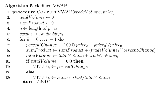
Figure 5.5.1 The vwapGain predictor Pseudocode |
Figure 5.5.2 shows a plot of the VWAP data (shown as blue dots). The value of the vwapGain predictor is the sum of the volume Weighted percent price changes, divided by the total volume. Show in Figure 5.5.2 is the 60 previous summary intervals.
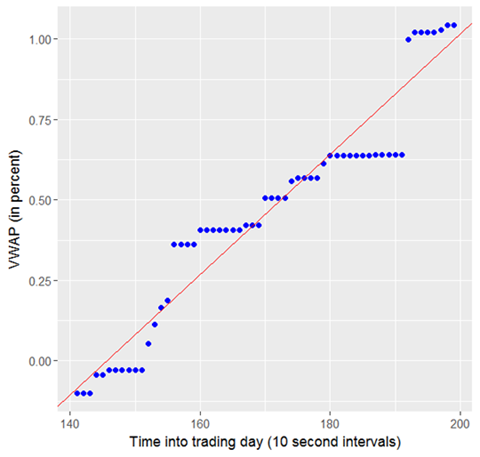
Figure 5.5.2 The vwapGain predictor |
Before discussing the current results, it is useful to compare the results that were obtained last year. Using these predictors, we were able to obtain the following results:
| Metric | TensorFlow | sklearn | H2O RF | H2O NN |
|---|---|---|---|---|
| accuracy | 0.6417 |
0.9086 |
0.9054 |
0.9193 |
| precision | 0.6218 | 0.5846 | 1.0000 | 1.0000 |
| recall | 0.7823 | 0.6726 | 0.6742 | 0.6750 |
| F1 | 0.6929 | 0.1255 | 0.3544 | 0.3903 |
| AUC | 0.6368 | 0.8580 | 0.8741 | 0.9203 |
| logloss | ---- | 3.1555 | 0.2354 | 0.2772 |
|
Figure 6.1 Results of first analysis |
When we began this analysis last year, we were warned that Machine learning analysis on financial dataset was very difficult. With this in mind, we had low expectations about obtaining good results.
This was our first attempt at analyzing the Bottle Rocket dataset, and we struggled to obtain only average results. At the time, we thought that the dataset was the problem. Surely our predictors were not the problem.
The next six months was spent looking for a way to improve the results. Then, we decided to try AutoML, and that led me to TPOT, auto-sklearn and H2O's AutoML.
The Jupyter notebook for the TPOT analysis (click here) was run under Windows 10 enterprise, release 17134.191, and Anaconda Python 3.6.5.
The first results from TPOT showed a great improvement. These Results showed that the Bottle Rocket dataset was not the problem. We noticed that TPOT created new predictors (features), and it also introduced a pipe-line model. We found that TPOT was very friendly to the sklearn package, and we could use many sklearn metrics to analyze the performance of the model.
The Jupyter notebook for Auto-sklearn (click here) was run on bash, version 4.3.48(1)-release (x86_64-pc-linux-gnu). This Lynux Shell is running Ubuntu 16.04.4 LTS, under Windows 10 enterprise, release 17134.191, and Anaconda Python 3.6.5.
The Jupyter notebook for H2O-AutoML (click here) was run under Windows 10 enterprise, release 17134.191, and Anaconda Python 3.6.5.
Clearly, H20 AutoML is a work-in-progress. We could not compute all the metrics we wanted (e.g. "recall"), and we observed that there are "issues" requesting the missing metrics.
The results are as follows:
| Metric | TPOT | auto-sklearn | H2O-AutoML |
|---|---|---|---|
| accuracy | 0.93925 | 0.91943799 | 0.88314970 |
| precision | 0.92127 | 0.89705603 | 1.00000000 |
| recall | 0.96143 | 0.94877461 | - |
| misclassification rate | 0.06075 | 0.880926 | 0.88092591 |
| F1 | 0.940922 | 0.92219076 | 0.88748788 |
| r2 | 0.75699 | 0.67773888 | 0.61682860 |
| AUC | 0.939108 | 0.91924997 | 0.95078805 |
| mse | 0.06075 | 0.08056201 | 0.09578897 |
| logloss | 2.09826 | 2.78255718 | 0.32046170 |
|
Figure 6.2 Results of second analysis |
After seeing the results of the AutoML optimization we realized:
We now regard the analysis we did last year as "first generation". Clearly, the results obtained by the AutoML packages are "second-generation".
The results obtained by TPOT are good enough to put into production. However, the production version is only used as an aid to an experienced day-trader (supervised). It is not good enough for "program trading" (un-supervised)
In day-trading, a false negative is not a disaster. It's unfortunate, but it doesn't affect the bottom line. However, a false positive does negatively affect profits. More work needs to be done on a scoring function that minimizes these trades.
AutoML packages that include feature engineering is where we will concentrate our efforts.